Linear Regression
Gilbert Berdine MDa, Shengping Yang PhDb
Correspondence to Gilbert Berdine MD. Email: gilbert.berdine@ttuhsc.edu
SWRCCC 2014;2(6):61-63
doi: 10.12746/swrccc2014.0206.077
...................................................................................................................................................................................................................................................................................................................................
I am analyzing data from a height and age study for children under 10 years old. I am assuming that height and age have a linear relationship. Should I use a linear regression to analyze these data?
...................................................................................................................................................................................................................................................................................................................................
In previous articles, statistical methods were presented which characterize data by a group mean and variance. The physical interpretation of this methodology is that the dependent variable has some average expected value (norm) and that deviations from the norm are due to random effects. Statistical methods were also discussed to compare two data sets and decide the likelihood that any differences were due to the random effects rather than systematic differences.
Some data have expected differences between two points. For example, it should surprise nobody that two children of different ages would have different heights. Suppose we wish to examine the nature of the effect of one variable, such as age, on another variable, such as height. We are not attributing the differences in height to some unknown random effect, such as imprecision in the birthdate, but we are expecting a difference in the dependent variable height due to an expected effect of the independent variable age.
Analysis starts with the examination of a scatter plot of the dependent variable on the y-axis and the independent variable on the x-axis.
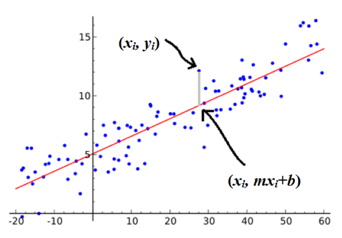
Figure 1 is adapted from a scatter plot in the Wikimedia Commons (1). The data points are the blue dots. Each point represents a pair of independent variable x value with its dependent variable y value. The red line is the regression line using slope intercept form:

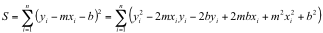
Every line can be defined by a slope (m) and y-intercept (b). Linear regression fits a “best” line to the set of data. What defines “best”? The most common method used to define “best” is the method of least squares. The “best” line is the line that minimizes the sum of the squares of the difference between the observed values for y and the predicted values m*x + b. The squares of the differences are used so that deviations below the line do not cancel deviations above the line. The sum of the variances (S) between the predicted values and observed values can be expressed as:
 .
.
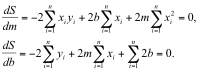
S is a function of the choices for both m and b. If a minimum value for a curve exists, the slope of the curve at that minimum is zero. The minimum value of S is determined by taking the derivative of S with respect to m and the derivative of S with respect to b and setting both expressions to zero. Note that during the calculation of the regression coefficients, the total variance is a function of the coefficients and the data values are treated as constants rather than variables.
Note that  where n is the number of data points.
This is a system of two equations with 2 unknowns, so a unique solution can be solved. The solution is usually shown in the following form:

The slope m is calculated first and is then used to calculate the intercept b. Note the symmetry in the formula for the slope m: both the numerator and denominator are the product of n and the sum of a product of individual values, minus the product of the sum of the first value and the sum of the second value. This form is common to all types of moment analysis. A complete discussion of moments is beyond the scope of this article.
Correlation
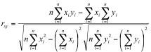
How good is the fit between the observed data and the parameterized linear model? The usual approach to answering this question is known as the Pearson Correlation Coefficient r. The Pearson r is a moment analysis known as covariance. For the population Pearson correlation coefficient, the general formula for  is:
is:

where σ is the standard deviation of a variable. The Pearson r is usually calculated from the same intermediate values used to calculate the regression coefficients:
 .
.
The Pearson r can have values from -1 to +1 with a value of 0 meaning no correlation at all, a value of +1 meaning perfect fit to a positive slope line and a value of -1 meaning perfect fit to a negative slope line. The special case of a perfect fit to a horizontal line also has r = 0, but this is because the dependent variable does not vary at all.
Example
Consider a simple set of 4 data points {(0, 1), (1, 3), (2, 5), (3, 7)}.
 = 0 + 1 + 2 + 3 = 6.
 = 1 + 3 + 5 + 7 = 16.
 = 0 + 1 + 4 + 9 = 14.
 = 1 + 9 + 25 + 49 = 84.
 = 0 + 3 + 10 + 21 = 34.
Slope m = [4 * 34 – 6 * 16] / [4 * 14 – 6 * 6] = [136 – 96] / [56 – 36] = 40 /20 = 2.
Intercept b = [16 – 2 * 6] / 4 = [16 – 12] /4 = 4 / 4 = 1.
The Pearson r = [4 *34 – 6 * 16] / √ [4 * 14 – 6 * 6] [4 * 84 – 16 * 16]
= [136 – 96] / √ [56 – 36] [336 – 256]
= 40 / √ [20 * 80] = 40 / √ [1600] = 40 /40 = 1.
Thus, we see a perfect fit to a line with positive slope.
Adaptations of Linear Regression
The main advantage of ordinary least squares is simplicity. The next advantage is that the math is well understood. This method can be easily adapted to non-linear functions.
The exponential function:
y = AeBx
can be adapted by taking the logarithm of both sides:
ln (y) = ln (A) + Bx.
By transforming y’ = ln (y) one can fit ln (y) to A and B. This is, in effect, drawing the data on semi-log graph paper and fitting the best line to the graph.
The power function:
y = AxB
can be analyzed in the same way:
ln (y) = ln (A) + B ln (x).
The graphical equivalence would be to plot the data on log-log paper and fit the best line to the result.
Multiple-regression adds parameters that need to be solved for best fit. Each new parameter adds an additional derivative expression that is set to zero and is part of a larger system of equations with the number of equations equal to the number of parameters. Generalized solutions of systems of equations are readily done with matrix notation that can be easily adapted to automated computing. This allows software packages to handle arbitrary numbers of parameters. An important caveat is that the parameters cannot be degenerate: that is parameters cannot be linear combinations of other parameters.
The method of ordinary least squares gives equal weight to all points based on the square of the deviation from best fit (variance). This method will tolerate small errors (residuals) in many points rather than larger errors (residuals) for a single point. Other best-fit models may work better for data sets where most points are good fits and a few points are outliers.
The generalized linear model method can be adapted to other types of data such as categorical data. The method of logistic regression will be presented in the next article.
References
- http://en.wikipedia.org/wiki/Linear_regression
- http://en.wikipedia.org/wiki/Pearson_product-moment_correlation_coefficient
- http://www.statisticshowto.com/how-to-find-a-linear-regression-equation/
- http://www.statisticshowto.com/how-to-compute-pearsons-correlation-coefficients/
...................................................................................................................................................................................................................................................................................................................................
Published electronically: 4/15/2014
Conflict of Interest Disclosures: None
Return to top